40 how to format data labels in excel charts
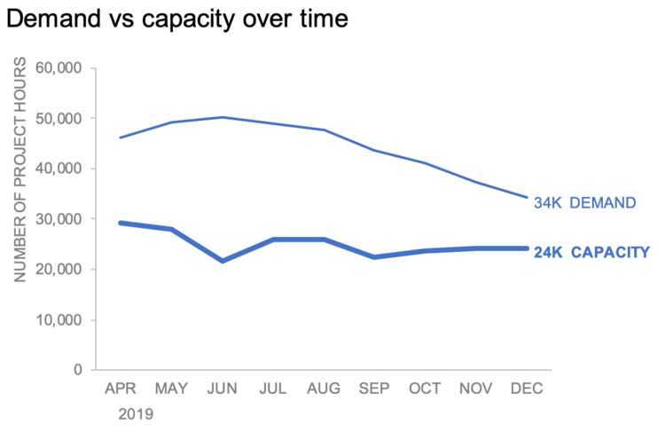
peltiertech.com › prevent-overlapping-data-labelsPrevent Overlapping Data Labels in Excel Charts - Peltier Tech May 24, 2021 · Overlapping Data Labels. Data labels are terribly tedious to apply to slope charts, since these labels have to be positioned to the left of the first point and to the right of the last point of each series. This means the labels have to be tediously selected one by one, even to apply “standard” alignments. Creating Conditional Data Labels in Excel Charts - YouTube We can make labels appear on our charts that don't have to do with the raw numbers that built the chart - and we can make them show up or not based on whatever conditions we want. In this...
chandoo.org › wp › change-data-labels-in-chartsHow to Change Excel Chart Data Labels to Custom Values? Now, click on any data label. This will select "all" data labels. Now click once again. At this point excel will select only one data label. Go to Formula bar, press = and point to the cell where the data label for that chart data point is defined. Repeat the process for all other data labels, one after another. See the screencast. Points to note:
How to format data labels in excel charts
How to create Custom Data Labels in Excel Charts - Efficiency 365 Two ways to do it. Click on the Plus sign next to the chart and choose the Data Labels option. We do NOT want the data to be shown. To customize it, click on the arrow next to Data Labels and choose More Options … Unselect the Value option and select the Value from Cells option. Choose the third column (without the heading) as the range. Formatting Charts in Excel - GeeksforGeeks 3. Formatting Data labels: You can add Data Labels by using the "+" button on the top right corner of the chart. Now open the Format Data Labels Window and can change the Font color, size, alignment, and many other options. 4. Formatting Data Series: You can change the color of the bar charts by selecting them and then open the "Format ... › blog › 2021/9/8How to format bar charts in Excel — storytelling with data Sep 12, 2021 · Another benefit of doing this is that now there’s enough space to pull the long data labels into the ends of the bars. This is just one of the decluttering steps we can take to reduce perceived cognitive burden. Here’s how to achieve this: 3. Click on any data label to highlight them all, then right-click and choose Format Data Labels:
How to format data labels in excel charts. Excel Charts - Aesthetic Data Labels - tutorialspoint.com To format the data labels − Step 1 − Right-click a data label and then click Format Data Label. The Format Pane - Format Data Label appears. Step 2 − Click the Fill & Line icon. The options for Fill and Line appear below it. Step 3 − Under FILL, Click Solid Fill and choose the color. › products › powerpointFormat Number Options for Chart Data Labels in PowerPoint ... Oct 21, 2013 · Alternatively, select the Data Labels for a Data Series in your chart and right-click (Ctrl+click) to bring up a contextual menu -- from this menu, choose the Format Data Labels option as shown in Figure 3. Figure 3: Select the Format Data Labels option Either of the above options will summon the Format Data Labels dialog box -- make sure that ... How to Use Cell Values for Excel Chart Labels - How-To Geek Select the chart, choose the "Chart Elements" option, click the "Data Labels" arrow, and then "More Options." Uncheck the "Value" box and check the "Value From Cells" box. Select cells C2:C6 to use for the data label range and then click the "OK" button. The values from these cells are now used for the chart data labels. Data Labels in Excel Pivot Chart (Detailed Analysis) Add a Pivot Chart from the PivotTable Analyze tab. Then press on the Plus right next to the Chart. Next open Format Data Labels by pressing the More options in the Data Labels. Then on the side panel, click on the Value From Cells. Next, in the dialog box, Select D5:D11, and click OK.
How to Add Two Data Labels in Excel Chart (with Easy Steps) Step 1: Create a Chart to Represent Data Step 2: Add 1st Data Label in Excel Chart Step 3: Apply 2nd Data Label in Excel Chart Step 4: Format Data Labels to Show Two Data Labels Things to Remember Conclusion Related Articles Download Practice Workbook Download this dataset and practice while going through this article. Add Two Data Labels.xlsx How to add or move data labels in Excel chart? - ExtendOffice In Excel 2013 or 2016. 1. Click the chart to show the Chart Elements button . 2. Then click the Chart Elements, and check Data Labels, then you can click the arrow to choose an option about the data labels in the sub menu. See screenshot: In Excel 2010 or 2007. 1. click on the chart to show the Layout tab in the Chart Tools group. See screenshot: 2. Then click Data Labels, and select one type of data labels as you need. See screenshot: Excel 2010: How to format ALL data point labels SIMULTANEOUSLY If you want to format all data labels for more than one series, here is one example of a VBA solution: Code: Sub x () Dim objSeries As Series With ActiveChart For Each objSeries In .SeriesCollection With objSeries.Format.Line .Transparency = 0 .Weight = 0.75 .ForeColor.RGB = 0 End With Next End With End Sub B brianclong Board Regular Joined Formatting Data Label and Hover Text in Your Chart - Domo In Chart Properties , click Data Label Settings. (Optional) Enter the desired text in the Text field. You can insert macros here by clicking the "+" button and selecting the desired macro. For more information about macros, see Data label macros. (Optional) Set the other options in Data Label Settings as desired.
› format-data-labels-in-excelFormat Data Labels in Excel- Instructions - TeachUcomp, Inc. Format Data Labels in Excel: Instructions To format data labels in Excel, choose the set of data labels to format. One way to do this is to click the "Format" tab within the "Chart Tools" contextual tab in the Ribbon. Then select the data labels to format from the "Current Selection" button group. ... how to add data labels into Excel graphs — storytelling with data To adjust the number formatting, navigate back to the Format Data Label menu and scroll to the Number section at the bottom. I'll choose Number in the Category drop-down and change Decimal places to 0 (side note: checking the Linked to source box is a good option if you want the labels to reformat when the formatting of the underlying source data changes). › en › resourcesHow to link charts in PowerPoint to Excel data :: think-cell When the source data for your data-driven charts is available in Excel, you can create charts directly from the Excel application. When data in Excel changes, you can either update the charts on command or have think-cell do the update automatically. 21.1 Creating a chart from Excel 21.2 Transposing linked data 21.3 Updating a linked element 21.4 How to add data labels from different column in an Excel chart? Right click the data series, and select Format Data Labels from the context menu. 3. In the Format Data Labels pane, under Label Options tab, check the Value From Cells option, select the specified column in the popping out dialog, and click the OK button. Now the cell values are added before original data labels in bulk. 4.
Formatting Charts
Excel tutorial: How to use data labels In this video, we'll cover the basics of data labels. Data labels are used to display source data in a chart directly. They normally come from the source data, but they can include other values as well, as we'll see in in a moment. Generally, the easiest way to show data labels to use the chart elements menu. When you check the box, you'll see ...
How to fix wrapped data labels in a pie chart - Excel Tips ...
Excel Chart - Selecting and updating ALL data labels The following procedure accomplished your requirement; tell me how it works out for you: - Right-click a "point" in the series, which actually will be a bar piece. - Choose add data labels. - Right-click again and choose format data labels. - Check series name. - Uncheck value.

Apply Custom Data Labels to Charted Points - Peltier Tech
Formatting data labels in Excel charts using VBA I would like to change the data labels for the picture below from decimals (0.8102), like that of the blue part, to percentage (81.02%), like the red part of the stacked chart. I have tried recording a macro but it does not show any code for the formatting of data labels.

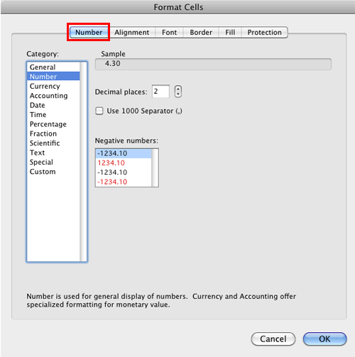
Format Number Options for Chart Data Labels in Excel 2011 for Mac
How to format the data labels in Excel:Mac 2011 when showing a ... Replied on December 7, 2015 Try clicking on Column or Row you want to set. Go to Format Menu Click cells Click on Currency Change number of places to 0 (zero) (if in accounting do the same thing. _________ Disclaimer:

How to Add Data Labels to an Excel 2010 Chart - dummies
Excel Custom Data Labels with Symbols that change Colors ... - YouTube In this tutorial we will learn how to format Data labels in Excel Charts to make them dynamically change their colors. And also how to insert any symbols in ...

microsoft excel - Adding data label only to the last value ...
Edit titles or data labels in a chart - support.microsoft.com The first click selects the data labels for the whole data series, and the second click selects the individual data label. Right-click the data label, and then click Format Data Label or Format Data Labels. Click Label Options if it's not selected, and then select the Reset Label Text check box. Top of Page

How to hide zero data labels in chart in Excel?
excel - Formatting chart data labels with VBA - Stack Overflow Here's the code so far: Sub FixLabels (whichchart As String) Dim cht As Chart Dim i, z As Variant Dim seriesname, seriesfmt As String Dim seriesrng As Range Set cht = Sheets ("Dashboard").ChartObjects (whichchart).Chart For i = 1 To cht.SeriesCollection.Count If cht.SeriesCollection (i).name = "#N/D" Then cht.SeriesCollection (i).DataLabels ...

How to: Display and Format Data Labels | WPF Controls ...
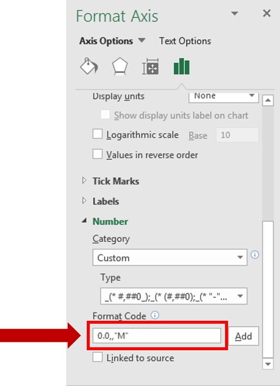
How to format axis labels individually in Excel - SpreadsheetWeb Double-click on the axis you want to format. Double-clicking opens the right panel where you can format your axis. Open the Axis Options section if it isn't active. You can find the number formatting selection under Number section. Select Custom item in the Category list. Type your code into the Format Code box and click Add button.

Adding Data Labels to Your Chart (Microsoft Excel)
Custom Chart Data Labels In Excel With Formulas - How To Excel At Excel Select the chart label you want to change. In the formula-bar hit = (equals), select the cell reference containing your chart label's data. In this case, the first label is in cell E2. Finally, repeat for all your chart laebls. If you are looking for a way to add custom data labels on your Excel chart, then this blog post is perfect for you.
Change the format of data labels in a chart
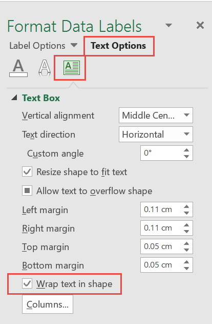
HOW TO CREATE A BAR CHART WITH LABELS ABOVE BAR IN EXCEL - simplexCT In the Format Data Labels pane, under Label Options selected, set the Label Position to Inside End. 16. Next, while the labels are still selected, click on Text Options, and then click on the Textbox icon. 17. Uncheck the Wrap text in shape option and set all the Margins to zero. The chart should look like this: 18.

How to Add Two Data Labels in Excel Chart (with Easy Steps ...
Custom Data Labels with Colors and Symbols in Excel Charts - [How To ... Step 4: Select the data in column C and hit Ctrl+1 to invoke format cell dialogue box. From left click custom and have your cursor in the type field and follow these steps: Press and Hold ALT key on the keyboard and on the Numpad hit 3 and 0 keys. Let go the ALT key and you will see that upward arrow is inserted. Hit 0 key. Then colon ; key.
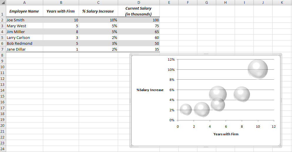
Add data labels to your Excel bubble charts | TechRepublic
› excel_data_analysis › excelExcel Data Analysis - Data Visualization - tutorialspoint.com Data Labels. Excel 2013 and later versions provide you with various options to display Data Labels. You can choose one Data Label, format it as you like, and then use Clone Current Label to copy the formatting to the rest of the Data Labels in the chart. The Data Labels in a chart can have effects, varying shapes and sizes.

Excel Charts - Aesthetic Data Labels
How to I rotate data labels on a column chart so that they are ... To change the text direction, first of all, please double click on the data label and make sure the data are selected (with a box surrounded like following image). Then on your right panel, the Format Data Labels panel should be opened. Go to Text Options > Text Box > Text direction > Rotate

Is it possible to conditionally format Data Labels on a ...
Change the format of data labels in a chart To format data labels, select your chart, and then in the Chart Design tab, click Add Chart Element > Data Labels > More Data Label Options. Click Label Options and under Label Contains , pick the options you want.

How to Add Total Data Labels to the Excel Stacked Bar Chart ...
How to Create Excel Charts (Column or Bar) with Conditional Formatting ... Step #1: Prep chart data. Step #2: Set up a column chart. Step #3: Modify the Overlap and Gap Width values. Step #4: Adjust the color scheme. Conditional formatting is the practice of assigning custom formatting to Excel cells—color, font, etc.—based on the specified criteria (conditions).

excel - How to show series-Legend label name in data labels ...
› blog › 2021/9/8How to format bar charts in Excel — storytelling with data Sep 12, 2021 · Another benefit of doing this is that now there’s enough space to pull the long data labels into the ends of the bars. This is just one of the decluttering steps we can take to reduce perceived cognitive burden. Here’s how to achieve this: 3. Click on any data label to highlight them all, then right-click and choose Format Data Labels:
how to add data labels into Excel graphs — storytelling with data
Formatting Charts in Excel - GeeksforGeeks 3. Formatting Data labels: You can add Data Labels by using the "+" button on the top right corner of the chart. Now open the Format Data Labels Window and can change the Font color, size, alignment, and many other options. 4. Formatting Data Series: You can change the color of the bar charts by selecting them and then open the "Format ...

Add data labels and callouts to charts in Excel 365 ...
How to create Custom Data Labels in Excel Charts - Efficiency 365 Two ways to do it. Click on the Plus sign next to the chart and choose the Data Labels option. We do NOT want the data to be shown. To customize it, click on the arrow next to Data Labels and choose More Options … Unselect the Value option and select the Value from Cells option. Choose the third column (without the heading) as the range.

Solved: How to show all detailed data labels of pie chart ...

Dynamic Number Format for Millions and Thousands - PK: An ...

Adding rich data labels to charts in Excel 2013 | Microsoft ...

How to Make an Excel Pie Chart
Dynamic Number Format for Millions and Thousands - PK: An ...

Change the format of data labels in a chart

Add data labels and callouts to charts in Excel 365 ...
Adding Data Labels To An Excel Chart | MyExcelOnline

How to Create a Pie Chart in Excel | Smartsheet
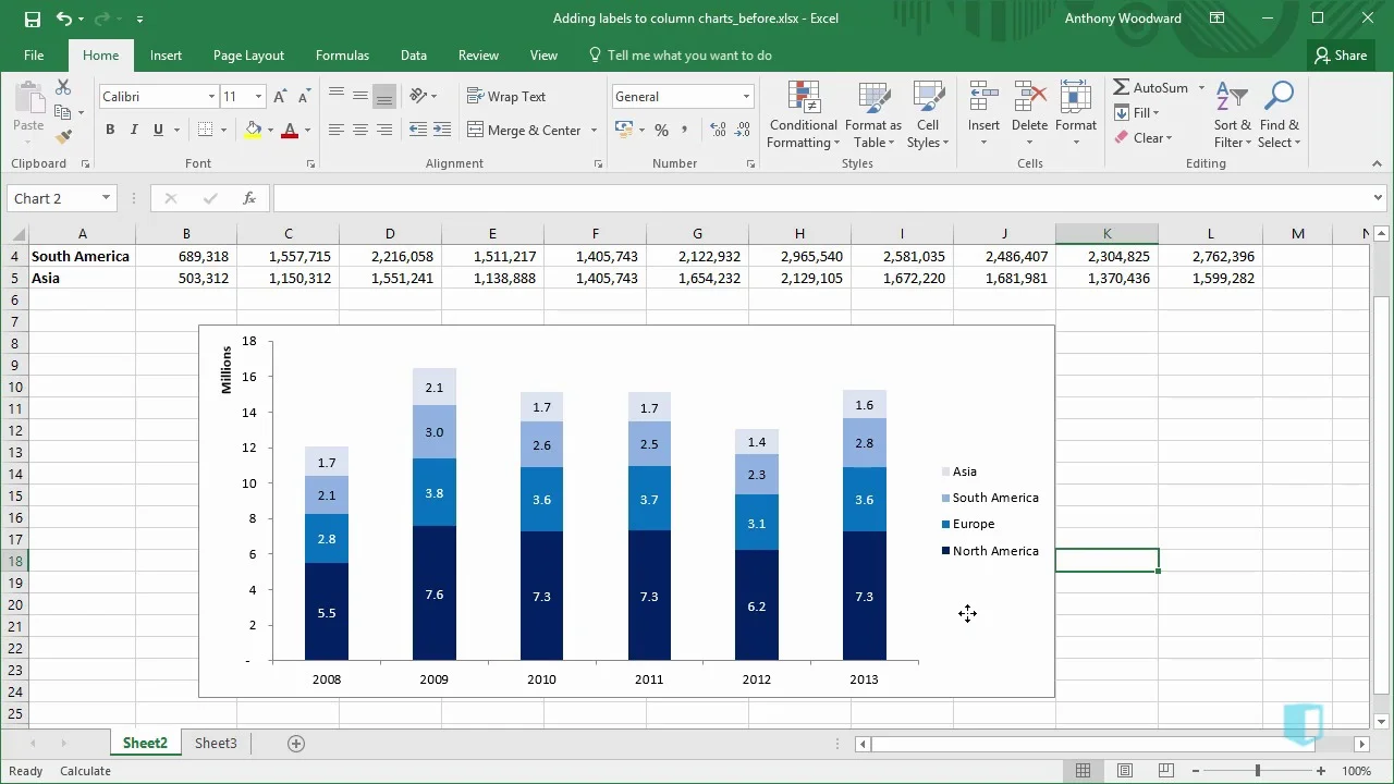
Adding Labels to Column Charts | Online Excel - KPMG Tax - Digital Now Course Training

How to set and format data labels for Excel charts in C#
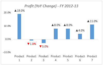
Color Negative Chart Data Labels in Red with downward arrow

Excel charts: add title, customize chart axis, legend and ...

Adding rich data labels to charts in Excel 2013 | Microsoft ...

Change the format of data labels in a chart

How to Use Cell Values for Excel Chart Labels

Enable or Disable Excel Data Labels at the click of a button ...

How to Add Data Labels to your Excel Chart in Excel 2013
Format Number Options for Chart Data Labels in Excel 2011 for Mac

How to show data labels in PowerPoint and place them ...

Add Labels ON Your Bars

Add or remove data labels in a chart
Post a Comment for "40 how to format data labels in excel charts"